I believe that true and deep understanding is the key to improve in any field of human activity.
I develop mathematical proofs to help achieve this goal.
The core of my activity is to create advanced mathematical tools to perform rigorous analysis of (variational) mathematical models.
Ideas and techniques I work with are from calculus of variations, geometric measure theory, optimal transport, and partial differential equations.
My research agenda focuses on tackling cutting-edge questions of modern science, and on creating an interdisciplinary research community that
overcomes the barriers of specialized languages and techniques.
Are you curious to know more about a project?
Do you work on similar questions, both from a experimental or theoretical point of view?
Contact me by email and I will be very happy to discuss with you!

Phase separation in composite materials - read about it
Self-assembly in polymers - read about it
Shape optimization - read about it
Epitaxial growth - read about it
Fine properties of denosining models - read about it
Recolorization of damaged images - read about it
Semi-supervised learning - read about it
The intricate microstructures of a material determine its macroscopic physical properties.
For instance, a soft material can be strengthened by adding microscopic pieces of a hard phase.
When the material posses different stable phases, it is not only the geometry of the microstructure that matters, but also the distribution of phases inside
the microstructure.
In order for practitioners to design specific materials enjoying desirable properties, it is therefore important to be able to understand the complex interaction
between these two process.
Derive analytically the effective macroscopic energies of fine mixtures of materials undergoing phase separation.
Standard models for phase separation assume the temperature of the medium to be uniform. There are situations though, where this is not the case. From the mathematical point of view the non-uniformity of the temperature could make the wells of the double well potential \(W\) be temperature dependent. We stress here that any other external field other than the temperature could cause the same effect. In order to model these cases Alt and Pawlow in [PH3] considered the following free energy:
\[ \int_\Omega \left[\frac{1}{\varepsilon} W(T(x), u(x)) + \varepsilon K(T(x))|\nabla u(x)|^2\right]\,dx, \]
where \(T \colon \Omega \to \mathbb{R}\) represents the temperature of the material (or any external field), and \(K\) is a given positive function. Here the unknowns
of the problem are both the temperature distribution \(T\) and the phase parameter \(u\). In particular, it could be the case where the wells of \(W\) depend themselves
on the temperature, and thus are not necessarily the same for all points \(x \in \Omega\).
The dependence of \(W\) on both of the unknowns poses analytical challenges.
In order to get some insight we assume the distribution of the temperature \(T\) to be given a priori and \(K\) to be constant.
These simplifications allow us to consider a free energy of the form
\[ \mathcal{F}_\varepsilon(u) := \int_\Omega \left[\frac{1}{\varepsilon} W(x, u(x)) + \varepsilon|\nabla u(x)|^2 \right]\,dx, \]
where the potential \(W \colon \Omega \times \mathbb{R}^M \to [0, \infty)\) is such that \(W(x, p) = 0\) if and only if \(p \in \{z_1(x), \dots, z_k(x)\}\), and the \(z_i \colon \Omega \to \mathbb{R}^M\) are given functions representing the stable phases of the material at each point \(x \in \Omega\). In this paper we consider for the first time the energy \(\mathcal{F}_\varepsilon\) in the vectorial case, with \(k \geq 2\), and for functions \(z_i\) which are possibly nonconstant. We are able, under suitable hypothesis on the potential \(W\) and on the wells \(z_1,\dots,z_k\) to identify the limiting energy:
\[ \mathcal{F}_0(u):=\int_{J_u} d_W(x, u^+(x), u^-(x))\,d\mathcal{H}^{N-1}(x) \]
if \(u\in BV(\Omega;\mathbb{R}^M) \) with \(u(x)\in \{z_1(x),\dots, z_k(x)\}\) for a.e. \(x\in\Omega\) and \(\infty\) otherwise in \(L^1(\Omega;\mathbb{R}^M) \). Here \(J_u\) denotes the jump of \(u\), \(u^+\) and \(u^-\) the traces of \(u\) on \(J_u\), and the function \(d_W:\Omega\times\mathbb{R}^M\times\mathbb{R}^M \to [0,\infty)\) is defined by\[ d_W(x,p,q):= \inf \left\{\int_{-1}^1 2\sqrt{W(x, \gamma(t))}|\gamma'(t)|\,dt \right\}, \]
where the infimum is taken over all \(W^{1,1}\) curves connecting \(p\) and \(q\).In this series of works, we investigate phase separation in a media with a periodic microstructure. We considered the case of liquid-liquid phase separation with the model
\[ \mathcal{F}_{\varepsilon,\delta}(u):=\int_{\Omega} \left[\, \frac{1}{\varepsilon}W\left(\frac{x}{\delta},u(x)\right) + \varepsilon|\nabla u(x)|^2 \,\right] \,dx\,. \]
Here \(\varepsilon, \delta>0\), \(W:\mathbb{R}^N\times\mathbb{R}^M\to[0,\infty)\) is a periodic potential that is \(Q\)-periodic in the first variable, where \(Q:=[0,1)^N\), such that \(W(x,p)=0\) if and only if \(p\in\{a,b\}\), for some \(a,b\in\mathbb{R}^M\). Our results are also valid for any other periodicity cell, and if the potential vanishes at several wells. We identified the limiting functional as \(\varepsilon\) and \(\delta\) vanishes, which is of the form
\[ \mathcal{F}_0(u):=\int_{\partial^* \{u=a\}} \sigma(\nu) d\mathcal{H}^{N-1} \]
if \(u\in BV(\Omega;\mathbb{R}^M)\) taking only the values \(a,b\), and \(\infty\) otherwise in \(L^1(\Omega;\mathbb{R}^M)\). Here \(\nu\) denotes the measure
theoretic normal to \(\partial^* \{u=a\}\).
We proved that the limiting energy density \(\sigma\) depends on the asymptotic behavior of the ratio \(\varepsilon/\delta\).
In particular, in [PH2] we studied the case \(\varepsilon/\delta\to+\infty\), we proved that \(\sigma\) is constant (namely, the limiting energy is isotropic)
and is the same as first sending \(\delta\to0\) and then \(\varepsilon\to0\).
When \(\varepsilon/\delta\to c\in(0,+\infty)\), we prove in [PH3] that \(\sigma\) is given by a cell problem, and is, in general, anisotropic.
Finally, we investigated the regime \(\varepsilon/\delta\to0\) in [PH4], where we proved that \(\sigma\) is anisotropic and is the same as first sending \(\delta\to0\) and
then \(\varepsilon\to0\).
In this paper, we investigate liquid-liquid phase separation in the case where there is a microscopic periodic microstructure and the wells of the potential depend
on the spatial position.
e identified a new scaling regime that leads to an asymptotic limiting energy that is of bulk type, not of a surface energy as in all the previous investigations.
In particular, we show that the model predicts microscopic, but not macroscopic phase separation.
More in detail, we consider the functional
\[ \mathcal{F}_{\varepsilon,\delta}(u):=\int_{\Omega} \left[\, \frac{\delta}{\varepsilon}W\left(\frac{x}{\delta},u(x)\right) + \frac{\varepsilon}{\delta}|\nabla u(x)|^2 \,\right] \,dx\,. \]
Here, \(W:\mathbb{R}^N\times\mathbb{R}^M\to[0,\infty)\) is a periodic potential that is \(Q\)-periodic in the first variable, where \(Q:=[0,1)^N\), such that \(W(x,p)=0\) if and only if \(p\in\{a(x),b(x)\}\), for some piecewise Lipschitz functions \(a,b:\Omega\to\in\mathbb{R}^M\), where we also allow for jumps of the wells and of the potential \(W\). We show that the limiting energy functional is given by
\[ \mathcal{F}_{0}(u):=\int_{\Omega} \left[\, \int_{J_{u(x,\cdot)}\cap Q} d_W(y, u^+(y), u^-(y))\,d\mathcal{H}^{N-1}(y) \,\right] \,dx\,, \]
where the limiting function \(u\in L^2(\Omega; BV(Q;\mathrm{R}^M))\).
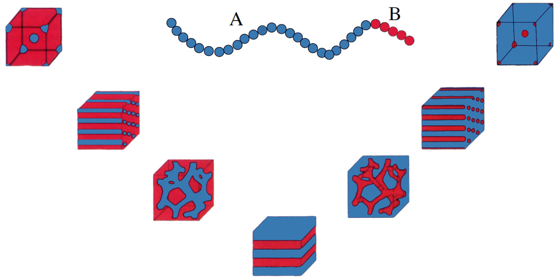
The extraordinary self-assembly property of block copolymers leads to the creation of astonishing patterns.
These beautiful examples of nature's regular shapes turn out to be extremely useful for applications (see [BC1] ).
Indeed, the usage of block copolymers in the bulk ranges from upholstery foam (as thermoplastic elastomer) to box tape, from asphalt additives to drug delivery, from
photonic crystals to nanoporus materials (see [BC1] , [BC2] ).
More recently, also thin films of diblock copolymers made their appearance in the industry sector (see [BC3] ).
Of particular interest is the possibility of accessing very small length scale not available to traditional litographic techniques.
Moreover, incorporating block copolymers into poly(ethylene oxide) may be useful in the construction of fuel cells and batteries.
All the applications of block copolymers require a high degree of control over the morphologies of stable configurations.
Investigate the landscape of patterns that (local) minimizers arrange into.
In particular, derive phase diagrams analytically in order to justify experimental
observations and design theory driven-experiments to explore new ranges of parameters.
We consider the sharp interface limit of the model introduced in 1986 by Ohta and Kawasaki (see [BC4] ) in the framework of the Density Functional Theory to describe the stable configurations of block copolymers. In this theory, a configuration is identified by a set \(E\subset \Omega\) where \(\Omega\subset\mathbb{R}^N\) is a bounded set representing the container. The set \(E\) is meant to represent the region where the density of the first monomer is negligible with respect to the other. The free energy reads as
\[ \mathcal{F}(E):=\mathcal{P}(E) + \gamma \int_E \int_E G(x,y) \,dx\,dy\,, \]
where \(G\) denotes the Greens function of \(-\triangle\) in \(\Omega\) with Neumann boundary conditions.
Here \(\gamma>0\) can be interpreted as the strength of the repulsion between the two monomers, and with \(\mathcal{P}(E)\) denote the perimeter of the set \(E\)
(the surface measure of \(\partial E\) in the case \(E\) is Lipschitz).
This model is a protoype for ground states created by the competition between a long-range repulsive force and a short-range attractive one.
In this paper we wanted to tackle the problem of determining the shape of (local) minimizers when the volume fraction of one phase is negligible with respect to the
other.
Experimental observations suggest that in this case the minority phase arrange into spherical droplets in a sea of the majority phase.
From the modeling point (see [BC6])
the shape of one connected component of the minority phase is described by (local) minimizers of the energy
\[ \mathcal{F}_\alpha(E):=\mathcal{P}(E) + \gamma \int_E \int_E \frac{1}{|x-y|^\alpha}\,dx\,dy\,, \]
for \(\alpha=N-2\). In this case \(E\subset\mathbb{R}^N\) and the contained \(\Omega\) plays no role anymore.
In order to study this limiting energy, in
[BC5]
we consider the energy \(\mathcal{F}_\alpha\) for the range of exponents \(\alpha\in(0,N-1)\).
From the physical point of view, this corresponds to consider a Riesz interaction energy in place of the Coulombic one.
We were able to prove that when \(\alpha\) is sufficiently small there exists a critical mass below which the only (up to translations) mass constrained minimizer of
the functional \(\mathcal{F}_\alpha\) is given by the ball, while for larger masses there is no existence, thus proving the above conjecture in this special case.
Moreover, we computed explicitly the threshold for local minimality of the ball, showing that it blows up as \(\alpha\to 0\). On the other hand, we show that the global
minimality threshold stays bounded as \(\alpha\to0\).
Local minimizers of the Ohta-Kawasaki functional satisfying a mass constrain are expected to reproduce what is observed in the experiments with diblock copolymers:
patterns that are (quasi) periodic at an intrinsic scale, with a structure depending strongly on the volume fraction of one phase with respect to the other, but that
is very closed to the one of a periodic surfaces with constant mean curvature (see [BC7]).
Proving analytically that (local) minimizers of the Ohta-Kawasaki functional enjoy this property is a formidable task.
A more reasonable, but still highly nontrivial, purpose is to exhibit a class of local minimizers that look like the observed configurations.
By using purely variational techniques, we proved that it is possible to find periodic critical points of the energy \(\mathcal{F}\) in the flat torus, whit a shape
closely resembling that of any given strictly stable periodic constant mean curvature surface. In particular, as observed in experiments, the intrinsic scale of
periodicity of these configurations depends on the weight \(\gamma\) multiplying the nonlocal term.
The behavior of polymers changes drastically when they are confined in thin films.
In particular, surface energy plays a more prominent role in such situation, as well as the thickness of film and the interaction with the substrate.
The goal of this paper is to study a two-dimensional model to describe this situation.
We identified the relaxed functional and we established regularity of locally minimizing partitions.
What is the long-range patterns in which diblock copolymers arrange into?
To shed some light into this questions, we consider a modification of the model describing the long-range interaction of spheres of the minority phase.
This latter is allowed to be a general concave function of the mass of each component.
We prove that in the plane, asymptotically, the optimal long-range arrangement is given by an hexagonal lattice.
It is often said that pattern formation is the result of the competition between terms with a different preference, like an attractive and a repulsive term.
A crucial question is how exactly different attractive and repulsive terms, and their interaction, affect the optimal shape.
Having a rigorous mathematical understanding of such mechanisms is of crucial importance for choosing the best terms to model a spe........
Understand the effect of the effect on the optimal shape of the interaction between attractive and repulsive terms.
\[ \min\{ \mathcal{F}(E) \,:\, |E|=m \}, \]
where the prototype of the attractive-repulsive interaction energy is given by
\[ \mathcal{F}(E) = \mathcal{E}_A(E) + \mathcal{E}_R(E). \]
Here, \(\mathcal{E}_A\) is the attractive term, while \(\mathcal{E}_R\) is the repulsive term.
The result of [BC5] can be stated as a stability result: for small values of \(\gamma\), the solution to the mass-constrained minimization problem
is still the solution in the case \(\gamma=0\).
What happens if the attractive term given by the isotropic perimeter is replaced by an isotropic perimeter?
It has been shown that if the anisotropy is regular enough (say, of class \(C^2\)), its Wulff shape is never a critical point.
In this paper we prove that if the anisotropy is crystalline, namely if its Wulff shape is given by a regular polytope (an \(N\)-dimensional version
of a regular polygon), then for small values of the mass \(\m\), it is still a solution to the mass constrained minimization problem.
In this paper, we focus only on the repulsive term. In particular, we want to answer the following question: the mass-constrained maximization problem
\[ \max\left\{ \int_E\int_E \frac{1}{|x-y|^\alpha} dx dy \,:\, |E|=m \right\} \]
is given by the ball (thanks to the rearrangement inequalities by Brascamp, Lieb, and Luttinger).
This can be viewed as follows: since the kernel of the non-local energy is isotropic, the solution is still isotropic.
Namely, the minimization problems selects the most symmetric object in the admissible class.
Is this also true if we restrict the class of admissible competitors?
In this work, we answer positively this question in the case where the kernel is a generalization of the Riesz kernel, and the
class of admissible competitors is the polygons with three or four sides.
Here we consider the case where both the attractive and the repulsive term are non-local, and given by potential kernels with exponents \(-\alpha\) and \(\beta\) respectively. Namely, we investigate the mass-constrained minimization problem
\[ \min\left\{ \int_E\int_E |x-y|^\beta dx dy + \int_E\int_E \frac{1}{|x-y|^\alpha} dx dy \,:\, |E|=m \right\}. \]
In this case, existence of a solution to the mass constrained minimization problem is not even guaranteed in the class of sets.
For this reason, we investigate the local minimality of the ball.
We prove that there exists an explicit threshold, depending on \(\alpha\) and \(\beta\), below which the ball is a local minimizer in the \(L^\infty\)
metric, and above which it is not stable.
In particular, we prove that the ball is never an \(L^1\) local minimizer.
In very few cases it is possible to obtain the explicit solution to a minimization problem. Especially if the solution is not one of the usual suspects. In this work, we provide the explicit solution when the attractive term is a quadratic kernel, while the repulsive is an anisotropic kernel:
\[ \min\left\{ \int_E\int_E |x-y|^2 dx dy + \int_E\int_E K(x-y) dx dy \,:\, |E|=m \right\}. \]
In dimension two and three, we show that the solution is an ellipse, with very few assumptions on the anisotropy.
In particular, the optimal ellipse is given by an semi-explicit expression, and tends to a ball as the mass increases.
Many important modern technologies, such as semiconductors, optoelectronics (quantum dot lasers), and magneto-optics, rely on the ability of controlling the growth
of a crystal over a substrate (see [EG1]).
In hetero-epitaxial growth (like InGaAs/GaAs or SiGe/Si), no stress free configurations exist, due to the lattice mismatch between the film and the rigid substrate.
Above a certain critical mass threshold, the flat profile becomes unstable (the Asaro-Tiller-Grinfeld instability, for single component crystals).
The stress is relieved via misfit dislocations, or morphological changes.
Here we focus on these latter.
They can be undulations of the profile, cusps, or formation of quantum dots (see figure below).
The specific properties of these morphological changes affect the features of the material.
It is therefore fundamental to be able to predict and to control the shape of the profile over the substrate.
Perform analytical studies of models describing the physics of crystal growth in order to direct the pattern formation of quantum dots.
In order to get a first insight in the understanding of the complex dynamics of surface diffusion with adatoms, we first consider the case where the elastic energy is neglected. This is physically reasonable in the small mass regime. In this case the evolution equations proposed by Fried and Gurtin in [EG2] read as
\[ \left\{ \begin{array}{ll} \partial_t u + (\rho+uH_{\partial E_t})V =D\Delta_{\partial E_t} \psi'(u) & \text{on } \partial E_t,\\ bV+\psi H-(\rho+uH_{\partial E_t})\psi'(u)=0 & \text{on } \partial E_t, \end{array} \right. \]
where \(\{E_t\}_{t\in (0,T)}\) are evolving smooth sets, \(V\) is the normal velocity to \(\partial E_t\), \(H_{\partial E_t}\) is its mean curvature,
\(u(\cdot,t):\partial E_t\rightarrow [0,\infty)\) is the adatom density on \(\partial E_t\), \(\rho > 0\) is the constant volumetric mass density of the crystal,
\(b>0\) is a constant called kinetic coefficient, and \(D>0\) is the diffusion coefficient of the adatoms.
The above system of equations has a variational nature, as it can be seen as a gradient flow (in a suitable norm) of the free energy
\[ \mathcal{F}(E,u):=\int_{\partial E} \psi(u) \,d \mathcal{H}^{N-1}\,. \]
Here \(E\subset\mathbb{R}^N\) represents the crystal, which is supposed to growth on a general shape, and \(\mathcal{H}^{N-1}\) denotes
the \((N-1)\)-dimensional Hausdorff measure.
A first study of the above system of equation is present in [EG3].
In this first paper we provided a rigorous study of the free energy \(\mathcal{F}\). In particular, the core of the work concerns the characterization of the relaxed functional of \(\mathcal{F}\) in a topology that allows us to take into consideration concentration and oscillation phenomena. It writes as
\[ \overline{\mathcal{F}}(E,\mu):= \int_{\partial^* E} \psi^{cs} (u) d\mathcal{H}^{N-1} + \Theta\mu^\perp(\mathbb{R}^N)\,, \]
where \(E\subset\mathbb{R}^N\) is the set of finite perimeter describing the crystal, \(\mu \) is a finite non-negative Radon measure and \(\mu= u \mathcal{H}^{N-1}\llcorner\partial^*E + \mu^\perp\) is its Radon-Nikodym decomposition. Moreover, \(\psi^{cs}\) denotes the convex sub-additive envelope of \(\psi\) and
\[ \Theta:=\lim_{t\to\infty} \frac{\psi^{cs}(t)}{t} \]
is the recession function of \(\psi^{cs}\), which is always finite since \(\psi^{cs}\) is at most linear at infinity.
Moreover, we explicitly solved the problem of minimizing the energy under a mass constraint, by proving that the only possible minimizing configurations
(as well as the only possible critical points) are balls with constant adatom density. Uniqueness, nevertheless, is not guaranteed in general.
From the numerical point of view it is important to have an model which can be simulated on a computer. We considered a phase field model used in [EG7] to perform numerical simulations in the special case \(\psi(t):=1+\frac{t^2}{2}\). Here we consider a general potential \(\psi\):
\[ \mathcal{F}_\varepsilon (\varphi, u) := \int_{\mathbb{R}^N} \left[\, \frac{1}{\varepsilon} W(\varphi) + \varepsilon|\nabla \varphi|^2 \,\right] \psi(u) d x, \]
where \(\varphi\in C^0(\mathbb{R}^N)\), \(u\in L^1(\mathbb{R}^N;[0,\infty))\), and \(W:\mathbb{R}\to[0,\infty)\) is a double well potential.
We proved convergence (in the sense of \(\Gamma\)-convergence) as \(\varepsilon\to0\) to the relaxed functional \(\overline{\mathcal{F}}\) we identified in
[EG5].
We were able to include the problem in a more general framework (that includes a large class of functionals) and proved results in this setting.
In this work we continue the study of the effect of adatoms by considering a two dimensional model of a crystal growth.
Starting from the same energy for regular configurations, we identify the relaxed energy when corrugations of the surface and creation of
vertical cracks take place.
If, on the one hand, the former phenomenon gives rise to the same relaxation effect on the energy, the latter leads to a different energy contribution on the crack.
Any image comes with an unavoidable distortion.
Indeed, external conditions other than defects or limitations of the instruments affect the quality of the acquired signal.
Therefore, before making use of the signal it is important to clean it in a reliable and efficient way.
The distortion is usually assumed to be the combination of a blurring effect and the addition of random noise.
Therefore, the original signal has to be recovered via an inverse problem, usually ill-posed.
To deal with such an issue it is nowadays customary to implementing a Bayesian approach based on a priori knowledge of the original signal and a maximum a
posteriori estimation.
This boils down to a minimization problem.
Establish rigorously fine properties of denoising models.
In the case the blurring effect is not present, a widely used variational technique for denoising a signal was proposed by Rudin, Osher and Fatemi in [DS1]. Their method is equivalent to recovering the clean signal \(u\in BV(I)\) by minimizing the functional
\[ \mathcal{F}(u):=|Du|(I) + \lambda\|u-f\|^2_{L^2(I)}\,, \]
where \(|Du|(I)\) denotes the total variation of \(u\) in the interval \(I\subset\mathbb{R}\), and \(f\in L^2(I)\) is the acquired signal.
Here \(\lambda>0\) is a parameter that controls the importance of the fidelity term over the regularisation one.
When \(\lambda\) is large the recovered signal \(u\) is expected to resemble the given signal \(f\).
On the other hand, when \(\lambda\) is very small, the regularisation effect of \(|Du|(I)\) prevails, and a constant signal is preferred in the
minimization procedure.
In this paper we consider the case where the initial data \(f\) is assumed to be a piecewise constant function.
The \(L^2\) norm is generalised to an \(L^p\) one, allowing for more flexibility in the choice of the fidelity term.
We are able to provide an analytic method to identify the solution of the minimization problem in the case \(p>1\) for all values of \(\lambda>0\).
The algorithm we propose is based on analytical results, and it is based on geometrical properties of the minimisers that allows to write explicitly the
Euler-Lagrange equation and to solve it.
We observe that in order to determine the solution of the minimization problem for a certain value \(\bar{\lambda}\) we have to solve several polynomial equation
whose number can be roughly bounded above by \(k(k+1)/2\), where \(k\) is the number of values assumed by the data \(f\).
What happens when the parameter \(\lambda\) of the ROF model moves? How do the property of the solutions change?
Well, when \(\lambda=0\) the solution is constant, while when \(\lambda\to\infty\), we get that the solution converges in \(L^2\) to the initial data \(f\).
Is there any monotonicity in this?
This is what we investigated in the paper. We proved, with a novel argument, that in the scalar case in dimension one, the jump set and the amplitude
of the jump are monotone with respect to the parameter \(\lambda\).
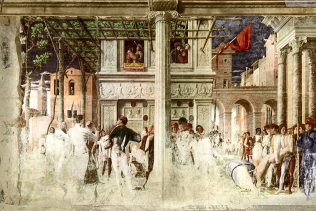
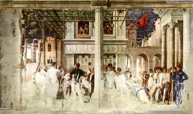
Restoring a damaged fresco is a challenging, fascinating and very important task to perform.
Mathematicians have proposed several strategies to suggest the best way to act on the painting.
The use of variational approach has been proven to be successful in this regards.
Other than simply act on the damaged region, these models also suggest way to improve the painting where colors is present, but maybe deteriorated.
Each model usually has an array of parameters that set the importance of each term in the energy, thus determining the weight of each term in the minimization procedure.
These are are usually manually tailored by practitioners for each specific image.
It is important to understand the effect of the interaction between the different parameters of the model and the features of the proposed restored image.
Moreover, it is auspicable to obtain a theoretical result allows to choose the optimal parameters for each given image, in order to reduce the need of
trial and error tests.
Provide practitioners with analytical methods for tuning the parameters of the model in order to obtain reconstructed images featuring specific properties.
The model we consider was used in [IM1] by Fornasier as a part of a project aimed at restoring the Mantegna's fresco in the Overtari Chapel in Padua. We are given a color image \(f\in L^p(\Omega;\mathbb{R}^M)\), \(M\geq1\) and \(p>1\), with a damaged region \(D\subset\Omega\) that consists in having the color removed. In this region we are left with a trace of the pre-existing color. This is modeled mathematically via a nonlinear distorsion \(\mathcal{L}\) of the color into a gray scale level, which is assumed to be of the form \(\mathcal{L}(u):= L(u\cdot e)\), where \(L:\mathbb{R}\to[0,\infty)\) is an increasing function (usually neither concave nor convex), and \(e\in\mathbb{R}^M\) is a unit vector chosen in such a way to best fit (i.e., with minimal total variance) the distribution of data from the real color. The optimal restored image \(u\in BV(\Omega;\mathbb{R}^M)\) is then obtained by minimizing the functional
\[ \mathcal{F}(u):=|Du|(\Omega)+\lambda\int_{\Omega\,\setminus \,D}|u-f|^p\,d x + \mu\int_D \bigl|\, L(u\cdot e)-L(f\cdot e) \,\bigr|^p\,d x\,. \]
Here \(p>1\), and \(|Du|(\Omega)\) denotes the total variation of the function \(u\) in \(\Omega\), acting as a regularizing term.
The parameters \(\lambda, \mu\) and the vector \(e\) are usually tuned according to the practitioner's experience.
The vectorial nature of the problem and the presence of the nonliner distorsion make this problem really challenging.
In this work we continued the analytic study initiated in [IM3] of the functional
proposed in
[IM1], without assuming perfect matching (i.e., \(\lambda,\mu < \infty\)).
We provided a general existence theorem as well as a characterization of the nonlinear distortion functions \(L\) giving rise to a nontrivial functional.
Finally, we considered the case where only a finite number of colors is available for the recolorization process (since, in practice, that is the case), and we
studied regularity properties of the minimizers.
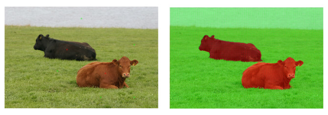
In the modern era, people are producing a tremendous amount of data.
To use them it is usually important to be able to partition them in classes according to some notion of similarity.
Variational models have been proved to be very successfully in performing this task.
Usually, each model possesses some parameters that practitioners vary in order to obtain better results for each particular case where the method is applied.
That there are very few theoretical results connecting the role of the parameters to the features of the partition one obtains by using that model.
Some of the parameters depend on the number of elements of the data set.
In order to evaluate the reliability of a labelling method it is important to understand whether the method is \emph{consistent} or not; namely it is desirable that
the minimization procedure approaches some limit minimization method when the number of elements of the data set goes to infinity.
This can help explain properties of the finite data method, and can also be used to justify, a posteriori, the use of a certain procedure in order to obtain specific
desired features of the partition.
Furthermore, understanding the large data limits can open up new algorithms.
Investigate analitically the consistency of variational algorithms for clustering of big data. Once the limiting model is identified, investigate the effect of
parameters on the limiting minimum partitions.
In this work we considered a variational model for clustering of point clouds that is a generalisation of the one studied by Thorpe and Theil in the case \(p=1\) (see
[BD2]), and by van Gennip and Bertozzi in [BD3] 4-regular graphs for \(N=2\) and \(p=2\).
A labeling of the data set \(X_n=\{x_i\}_{i=1}^n\subset\mathbb{R}^N\) is a function \(u:X_n\to\{c_1,\dots,c_k\}\), where \(c_1,\dots,c_k\in\mathbb{R}^M\) are the classes we want to partition the point cloud into.
For numerical reasons, we allow for soft classification, namely we consider labels \(u:X_n\to\mathbb{R}^M\) and we penalise more and more, as \(n\to\infty\), labels that do not agree with
\(c_1,\dots,c_k\).
The discrete functional \(\mathcal{G}_n:L^1(X_n)\to[0,\infty]\) reads as
\[ \mathcal{G}_n(u):= \frac{1}{\varepsilon_n n^2} \sum_{i,j=1}^n W_n^{ij} |u(x_i) - u(x_j)|^p +\frac{1}{\varepsilon_n n} \sum_{i=1}^n V(u(x_i)) \\ \]
Here \(W_{ij}^n\) are the weights between \(x_i\) and \(x_j\), and the non-negative function \(V\) vanishes only on the set \(\{c_1,\dots,c_k\}\).
The main result of the paper is the consistency of the model \(\mathcal{G}_n\).
Namely, we prove that the functional \(\mathcal{G}_n\) \(\Gamma\)-converges to a limiting functional we explicitly identified.
This turns out to be an anisotropic perimeter functional with density.